What Is Binomial Distribution?
Binomial distribution is a discrete probability distribution that models the number of successes in a fixed number of independent trials, where each trial produces exactly one of two outcomes and the probability of success stays the same throughout. Named after the binomial theorem — which Jacob Bernoulli formalized in Ars Conjectandi (1713), building on earlier work by Blaise Pascal — it became the foundation of modern probability theory.
The key word is counting. You are not asking "what is the probability of one coin landing heads?" You are asking "what is the probability of getting exactly 7 heads in 10 tosses?" That counting question is precisely what binomial distribution answers.
Binomial distribution is a discrete probability distribution that models the number of successes in a fixed number of independent trials, where each trial has exactly two outcomes and the probability of success remains constant. It is defined by two parameters: n (number of trials) and p (probability of success per trial). Written X ~ B(n, p).
🔑 Key Takeaways
The most important points to understand before working with binomial distribution.
Binomial distribution counts successes, not single-event probabilities. It answers "how many times?" over n repeated trials.
All four BINS conditions must be met. A single violated condition invalidates the model entirely.
The distribution is discrete. X can only equal 0, 1, 2, ..., n — never a fraction.
Mean = np; variance = np(1−p); mode = ⌊(n+1)p⌋. These three formulas describe the center, spread, and peak without computing the full PMF.
Bernoulli distribution is binomial with n = 1. Every Bernoulli trial is the atomic unit of a binomial experiment.
The 10% rule allows binomial for sampling without replacement — provided the sample is smaller than 10% of the total population.
The 4 Conditions for Binomial Distribution

The BINS conditions: Binary outcomes, Independent trials, fixed Number of trials, and Same probability of success.
Before applying the binomial model, check all four conditions. A single violated condition means the model will give wrong answers — no matter how carefully you apply the formula afterward.
Fixed Number of Trials
The number of trials n is set in advance and does not change. You flip a coin exactly 20 times, not "until you get 5 heads."
Independent Trials
The outcome of one trial does not affect any other. Drawing cards with replacement is independent; drawing without replacement generally is not.
Binary Outcomes Only
Each trial ends in exactly one of two outcomes: success or failure. Everything that is not "success" counts as "failure."
Constant Probability
The probability of success p is identical on every trial. A fair coin always has p = 0.5, trial after trial.
Memory Aid: The BINS Acronym
Binary outcomes
Each trial has exactly two outcomes: success or failure.
Independent trials
Trials do not influence each other in any way.
Number of trials is fixed
n is determined before the experiment begins.
Same probability each trial
p remains constant across all n trials.
The 10% Rule: When Sampling Without Replacement Is Acceptable
Strict independence requires sampling with replacement. But in practice, many surveys and quality-control checks sample without replacement from a finite population. The 10% rule provides a practical workaround:
The binomial model is an acceptable approximation for sampling without replacement provided the sample size is no more than 10% of the total population. When n ≤ 0.10 × N (population size), the change in p after each draw is small enough to be safely ignored. When n > 10% of N, use the hypergeometric distribution instead.
Example: Polling 50 voters from a city of 100,000. The sample (50) is 0.05% of the population — well under 10% — so the binomial model applies. But drawing 5 cards from a 20-card deck (sample = 25% of population) violates the rule; there the hypergeometric distribution is correct. See the study design guide for a full discussion of sampling methods.
Sample exceeds 10% of population without replacement? Use hypergeometric distribution. No fixed n (counting events per hour)? Use Poisson distribution. Counting trials until the first success? Use geometric distribution.
Binomial Distribution Formula (PMF)
The probability mass function (PMF) gives the probability of observing exactly k successes in n trials. This is the formula you will use for most direct calculations.
n = number of trials
k = number of successes
p = P(success on one trial)
1−p = P(failure on one trial)
C(n,k) = number of ways to arrange k successes
Each of the three parts does distinct work. The binomial coefficient C(n,k) counts every possible arrangement of k successes among n positions. The term pk gives the probability those k trials are all successes. And (1−p)n−k gives the probability the other n−k trials are all failures. Multiply them together because all three must happen simultaneously.
Complete Probability Distribution Table: b(5, 0.25)
To see the full shape of a binomial distribution at once, compute P(X = k) for every value of k from 0 to n. Here is the complete distribution for n = 5 trials, p = 0.25 (a coin that shows heads 25% of the time):
| k (successes) | C(5,k) | pk | (1−p)5−k | P(X = k) | Visual |
|---|---|---|---|---|---|
| 0 | 1 | 1.0000 | 0.2373 | 0.2373 | |
| 1 | 5 | 0.2500 | 0.3164 | 0.3955 | |
| 2 | 10 | 0.0625 | 0.4219 | 0.2637 | |
| 3 | 10 | 0.0156 | 0.5625 | 0.0879 | |
| 4 | 5 | 0.0039 | 0.7500 | 0.0146 | |
| 5 | 1 | 0.0010 | 1.0000 | 0.0010 |
The highlighted row (k = 1) is the mode — the most likely outcome. Probabilities sum to 1.0000. Notice the right skew: with p = 0.25, low counts are more probable than high ones. Use the binomial distribution calculator to generate tables for any n and p instantly.
Cumulative Distribution Function (CDF)
The CDF answers "what is the probability of at most k successes?" by summing the PMF from 0 to k:
Use the PMF when you need the probability of exactly k successes. Use the CDF when you need the probability of k successes or fewer. For "at least k" probabilities, compute 1 − P(X ≤ k−1). For "more than k," compute 1 − P(X ≤ k).
Mean, Variance, Mode & Standard Deviation
You do not need the full PMF to describe a binomial distribution. Four summary statistics — derived directly from n and p — capture its center, spread, and peak.
If you flip a fair coin 100 times, the mean is 100 × 0.5 = 50 heads. The variance is 100 × 0.5 × 0.5 = 25, and the standard deviation is 5. On a typical run, you would land within one standard deviation of the mean — between 45 and 55 heads — about 68% of the time.
Mode and Median of Binomial Distribution
Mode = ⌊(n+1)p⌋. When (n+1)p is exactly an integer, there are two modes: (n+1)p and (n+1)p − 1. Special cases: mode = 0 when p = 0; mode = n when p = 1.Example: For B(10, 0.3): (10+1)×0.3 = 3.3, so mode = ⌊3.3⌋ = 3. For B(9, 0.4): (9+1)×0.4 = 4.0 (integer), so there are two modes: 4 and 3.
|median − np| ≤ 1. When np is an integer, the mean, median, and mode all coincide at np. For non-integer np, the median is usually round(np).
γ₁ = (1 − 2p) / √(np(1−p)). Zero when p = 0.5 (symmetric). Positive (right-skewed) when p < 0.5. Negative (left-skewed) when p > 0.5.
If X ~ B(n, p) and Y ~ B(m, p) are independent with the same p, then X + Y ~ B(n+m, p). The binomial distribution is closed under addition when p is constant. This property underpins pooled significance tests and sequential sampling designs.
How to Calculate Binomial Probability: Step by Step
Calculating binomial probabilities follows a repeatable six-step process. Work through each step in order and the formula becomes mechanical — no guesswork required.
A fair coin is flipped 8 times. What is the probability of getting exactly 3 heads?
Identify parameters: n = 8 (total flips), k = 3 (heads wanted), p = 0.5 (fair coin), q = 1 − 0.5 = 0.5
Compute C(8,3): 8! / (3! × 5!) = (8 × 7 × 6) / (3 × 2 × 1) = 336 / 6 = 56
Compute pk: 0.53 = 0.125
Compute (1−p)n−k: 0.55 = 0.03125
Multiply: P(X = 3) = 56 × 0.125 × 0.03125 = 56 × 0.00390625 = 0.2188
Check mode: Mode = ⌊(8+1)×0.5⌋ = ⌊4.5⌋ = 4. Getting 3 heads is one below the most likely result.
Answer: There is a 21.9% probability of getting exactly 3 heads in 8 coin flips.
A drug trial shows a 70% success rate. If 10 patients receive the drug, what is the probability that exactly 7 respond?
Identify parameters: n = 10, k = 7, p = 0.70, q = 0.30. Check BINS conditions: fixed n ✓, independent patients ✓, binary outcome ✓, constant p ✓.
Compute C(10,7): 10! / (7! × 3!) = (10 × 9 × 8) / 6 = 720 / 6 = 120
Compute p7: 0.707 = 0.0823543
Compute (0.30)3: 0.027
Multiply: P(X = 7) = 120 × 0.0823543 × 0.027 ≈ 120 × 0.002223 ≈ 0.2668
Answer: There is approximately a 26.7% probability that exactly 7 of the 10 patients respond. Mean = 10 × 0.70 = 7 patients. Mode = ⌊(11)×0.70⌋ = ⌊7.7⌋ = 7. Variance = 10 × 0.70 × 0.30 = 2.1.
A factory line has a 5% defect rate. In a batch of 20 items, what is the probability that at most 2 items are defective?
Identify parameters: n = 20, p = 0.05, q = 0.95. We need P(X ≤ 2) = P(X=0) + P(X=1) + P(X=2).
P(X=0): C(20,0) × 0.050 × 0.9520 = 1 × 1 × 0.3585 = 0.3585
P(X=1): C(20,1) × 0.051 × 0.9519 = 20 × 0.05 × 0.3774 = 0.3774
P(X=2): C(20,2) × 0.052 × 0.9518 = 190 × 0.0025 × 0.3972 = 0.1887
Sum all three: P(X ≤ 2) = 0.3585 + 0.3774 + 0.1887 = 0.9246
Answer: There is a 92.5% probability that a batch of 20 items contains 2 or fewer defectives. Mean = 20 × 0.05 = 1 defect. Mode = ⌊21 × 0.05⌋ = ⌊1.05⌋ = 1.
Sample Proportions: From Count to Percentage
When a binomial count X is divided by the number of trials n, the result is the sample proportion p̂ = X/n. This converts the count of successes into a percentage, which is often more interpretable — and is the basis for confidence intervals and hypothesis tests about proportions.
Distribution of the Sample Proportion p̂ = X/n
Since X ~ B(n, p), we can derive the properties of p̂ directly from the properties of X:
The standard deviation of p̂ is called the standard error of the proportion. As n increases, the standard error shrinks — larger samples give more precise estimates of p. This is the foundation behind the confidence interval for a proportion.
Worked example: A poll of 500 voters finds 210 support Candidate A. Here p̂ = 210/500 = 0.42. The standard error is √(0.42 × 0.58 / 500) = √0.000487 ≈ 0.022. So the estimated true proportion is 0.42 ± 0.022 at roughly one standard error. See confidence intervals and proportion hypothesis testing to take this further.
Calculating Binomial Probability in Excel, Python & R
For large n values, manual calculation becomes tedious. Every major statistical software package has built-in binomial functions that handle the arithmetic in one line.
Excel
=BINOM.DIST(k, n, p, FALSE)
' CDF — probability of k or fewer successes
=BINOM.DIST(k, n, p, TRUE)
' Example: P(X = 7) with n=10, p=0.7
=BINOM.DIST(7, 10, 0.7, FALSE) → 0.2668
' Inverse: smallest k such that P(X ≤ k) ≥ 0.95
=BINOM.INV(n, p, 0.95)
Python (SciPy)
# PMF — exactly k successes
binom.pmf(7, n=10, p=0.7) # → 0.2668
# CDF — at most k successes
binom.cdf(7, n=10, p=0.7) # → 0.6172
# Mean, variance, std deviation
binom.mean(n=10, p=0.7) # → 7.0
binom.var(n=10, p=0.7) # → 2.1
binom.std(n=10, p=0.7) # → 1.449
# Full PMF table for k = 0 to 10
[binom.pmf(k, n=10, p=0.7) for k in range(11)]
R
dbinom(7, size=10, prob=0.7) # → 0.2668
# CDF — at most k successes
pbinom(7, size=10, prob=0.7) # → 0.6172
# Generate a full PMF table k = 0 to 10
dbinom(0:10, size=10, prob=0.7)
# Exact binomial test (one-sample)
binom.test(x=61, n=100, p=0.5)
Properties and Shape of Binomial Distribution
The shape of a binomial distribution is determined entirely by n and p. Understanding how these parameters control the shape lets you visualize outcomes before calculating a single probability.
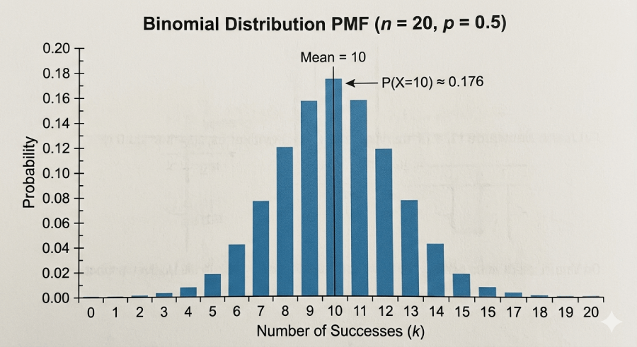
Symmetric binomial distribution (n = 20, p = 0.5). The peak occurs at the mean (np = 10), with equal spread on both sides.
| Parameter Combination | Shape | Skewness Direction | Typical Scenario |
|---|---|---|---|
| p = 0.5 | Symmetric, bell-like | None (zero skewness) | Fair coin flips |
| p < 0.5 | Right-skewed | Positive skew | Rare disease diagnosis, defects |
| p > 0.5 | Left-skewed | Negative skew | High-accuracy tests, drug response |
| Large n, any p | Approaches normal | Near zero | Large-sample quality control |
| Very small p, large n | Right-skewed, sparse | Strong positive | Manufacturing rare defects |
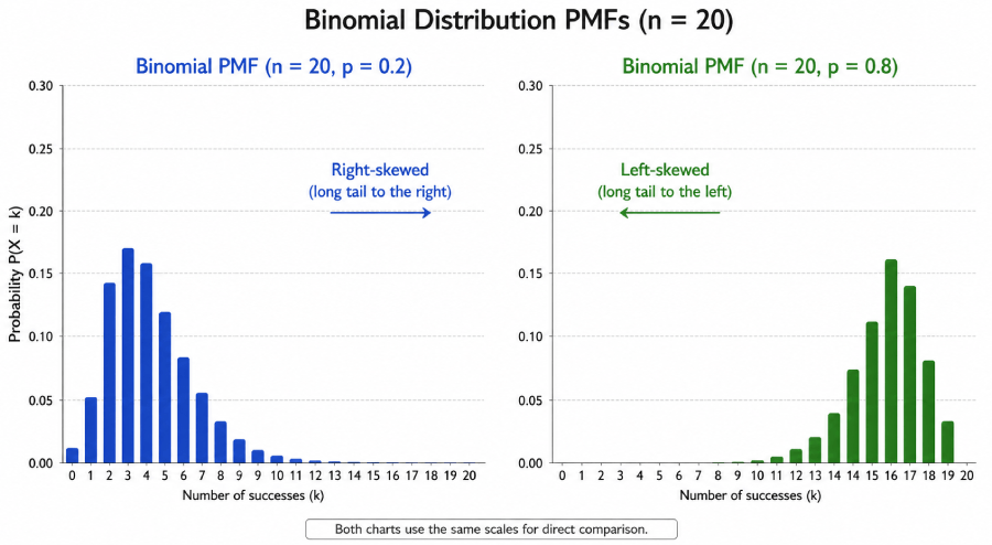
Right-skewed distribution (p = 0.2). Most outcomes cluster near 0, with a long tail to the right.
As n grows large, the binomial distribution smooths out and begins to look like a bell curve — this is the Central Limit Theorem in action. The bars of the probability distribution become narrower relative to the spread, concentrating around the mean. You can explore these shapes interactively with the bell curve generator and the central limit theorem page.
Binomial Test: Is This Result Statistically Significant?
The binomial test is a one-sample significance test that uses the binomial distribution to decide whether an observed number of successes is consistent with a claimed probability p₀ under the null hypothesis. It is the natural test whenever you have a binary outcome and a known or claimed rate to compare against.
Worked Example: Is This Coin Fair?
A coin is flipped 100 times and lands heads 61 times. At the 5% significance level, is there evidence the coin is unfair?
The binomial test is particularly useful when sample sizes are small and the normal approximation is not reliable. In R, use binom.test(x, n, p). In Python, use scipy.stats.binomtest(k, n, p). For A/B testing applications, the A/B test calculator applies the same binomial logic to conversion rate experiments. See the hypothesis testing guide for the full framework.
Real-Life Applications of Binomial Distribution
The binomial model appears wherever outcomes are binary and trials repeat under controlled conditions. Below are five fields where it drives actual decisions.
Medicine & Clinical Trials
A drug has a 65% response rate. Out of 15 patients in a pilot study, what is the probability that at least 10 respond? Binomial distribution gives the exact probability needed for go/no-go decisions.
Quality Control
A factory accepts a shipment if fewer than 3 items in a sample of 50 are defective. With a known defect rate of 4%, binomial tells you the probability of passing — or failing — that inspection.
Finance & Risk
Credit analysts model loan defaults as independent Bernoulli trials. Binomial distribution estimates the probability that k of n borrowers in a portfolio default within a year.
Machine Learning & A/B Testing
In A/B testing, user conversions are binomial. With n visitors and a click-through rate p, binomial distribution backs the statistical significance tests used to declare a winner.
Sports Analytics
A baseball player with a .300 batting average has a 30% probability of a hit on each at-bat. In a 10-at-bat game, binomial distribution predicts the probability distribution of his hits that day.
Real-World Example
COVID-19 Vaccine Efficacy Trials
In Phase III vaccine trials, each participant is treated as an independent trial with two outcomes: infection or no infection. With tens of thousands of participants and a known background infection rate, binomial (and related) models compute the probability of observing the recorded number of infections under a null hypothesis of no vaccine effect. The resulting p-values drove the emergency authorization decisions that shaped global public health policy in 2020 and 2021. For a deeper dive, see the hypothesis testing in clinical trials article and the randomized controlled trials guide.
Binomial vs. Poisson vs. Normal Distribution
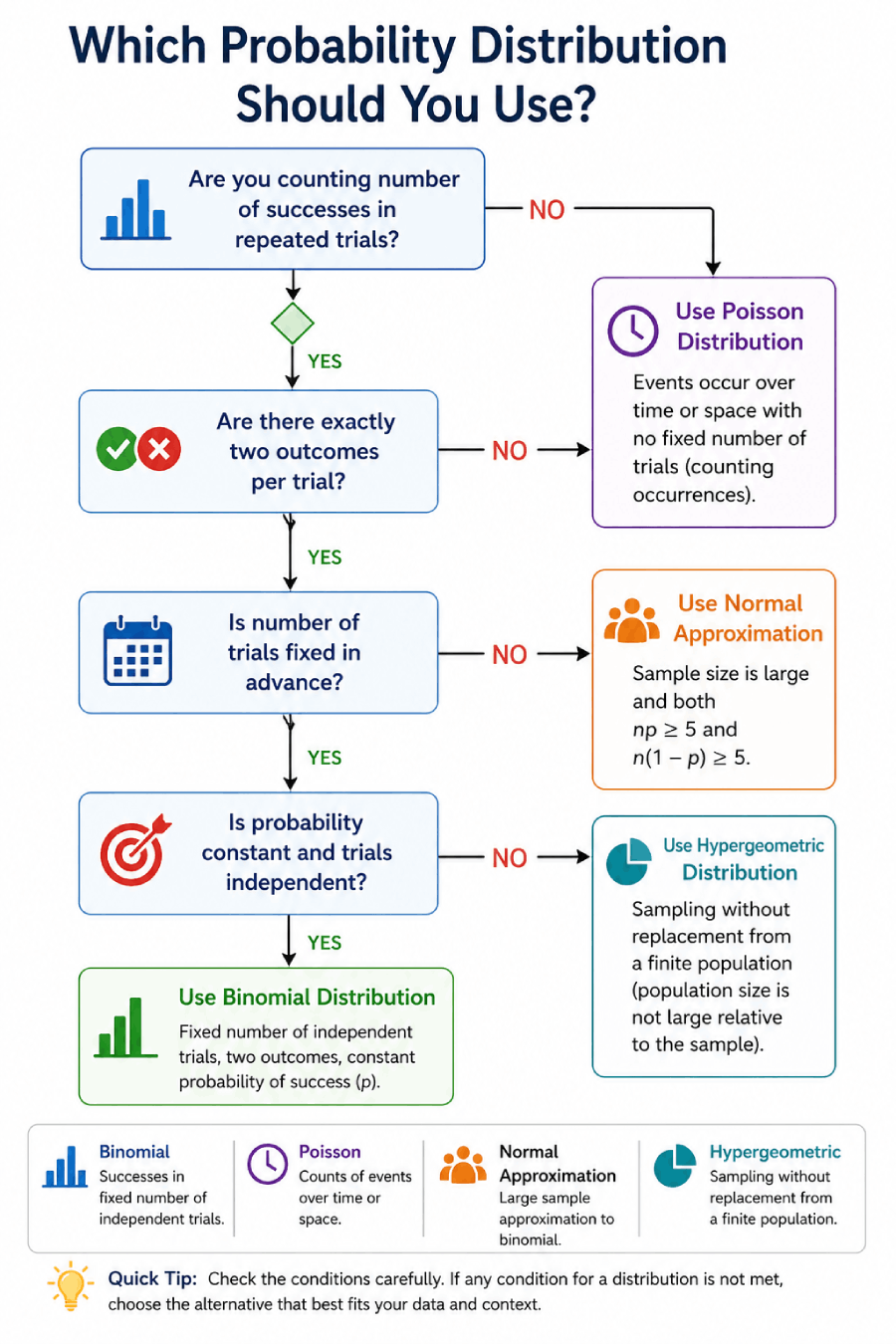
Decision flowchart for selecting between binomial, Poisson, normal, and hypergeometric distributions.
The three distributions most commonly confused with the binomial all occupy neighboring territory in probability theory. The table below separates them clearly. For deeper exploration, the normal distribution guide and the statistics and probability overview cover the mathematical relationships in detail.
| Attribute | Binomial | Poisson | Normal |
|---|---|---|---|
| Type | Discrete | Discrete | Continuous |
| Parameters | n, p | λ (rate) | μ, σ |
| Number of trials | Fixed (n known) | Not fixed (or very large) | N/A |
| Possible values of X | 0, 1, 2, ..., n | 0, 1, 2, ... (no upper bound) | Any real number |
| Mean | np | λ | μ |
| Variance | np(1−p) | λ | σ² |
| Mean = Variance? | Only when p = 0 | Always (μ = σ²) | No relationship |
| Mode | ⌊(n+1)p⌋ | ⌊λ⌋ or ⌊λ⌋−1 | μ (same as mean) |
| Best used when | Fixed n, binary outcomes, constant p | Rare events, large n, small p, np = λ | Continuous data, large n (CLT) |
| Example | Defects in 50 units | Calls per hour at a call center | Heights, measurement errors |
Binomial to Poisson: The Limiting Relationship
As n → ∞ and p → 0, while the product λ = np stays constant, the binomial distribution converges to Poisson(λ). In practice, if n ≥ 20 and p ≤ 0.05 — or n ≥ 100 and np ≤ 10 — the Poisson approximation is accurate and far easier to compute. The Poisson distribution guide documents the full derivation of this limit.
Binomial to Normal: The Approximation Rule
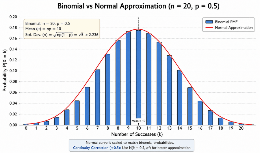
Binomial distribution (bars) overlaid with its normal approximation (curve). The fit improves as n becomes larger and both np and n(1−p) are sufficiently large.
When both np ≥ 5 and n(1−p) ≥ 5, the binomial distribution is well-approximated by N(np, np(1−p)). Add a continuity correction of ±0.5 to account for the shift from discrete to continuous: for example, to find P(X ≤ 8) with the normal approximation, evaluate P(Y ≤ 8.5) where Y is normal. This approximation is why the normal distribution is so central to large-sample binomial inference. You can verify critical values using the Z-table and find the approximation quality with the normal approximation calculator.
Fixed n, binary outcomes, constant p → Binomial. Rare events, large or unknown n, small p → Poisson. np ≥ 5 and n(1−p) ≥ 5 → approximate with Normal. Sampling without replacement and n > 10% of population → Hypergeometric.
Common Mistakes When Using Binomial Distribution
These five errors appear repeatedly in statistics courses and applied work. Each one produces incorrect probabilities — sometimes dramatically so.
Ignoring the 10% Rule When Sampling Without Replacement
Drawing 5 cards from a 52-card deck without replacement changes p after each draw. When the sample exceeds 10% of the population, independence fails and the binomial model is wrong. Use hypergeometric distribution, or check the 10% rule first.
Confusing P(X = k) with P(X ≤ k)
These are completely different quantities. P(X = 3) is the probability of exactly 3 successes. P(X ≤ 3) sums all probabilities from 0 to 3. Mixing them up produces answers that can be off by a factor of 3 or more.
Applying Binomial When p Is Not Constant
If a player's scoring probability changes depending on whether the game is home or away, p is not constant across trials. A weighted mixture of distributions, not a single binomial, models this correctly.
Forgetting to Verify All Four BINS Conditions First
Many students jump straight to the formula without checking BINS. A single violated condition invalidates the model. The formula will still produce a number — but that number will be wrong.
Using Binomial When n Is Not Fixed
"Count calls until you get 3 complaints" — this has no fixed n. The number of trials is itself a random variable. This is a negative binomial (or Pascal distribution) problem, not binomial.
Summary: Binomial Distribution Quick Reference
| Property | Formula / Value | Notes |
|---|---|---|
| Notation | X ~ B(n, p) | n = trials, p = success probability |
| Support | k = 0, 1, 2, ..., n | Discrete — only whole numbers |
| PMF | C(n,k) × pk × (1−p)n−k | Probability of exactly k successes |
| CDF | Σ P(X=i) from i=0 to k | Probability of k or fewer successes |
| Mean | μ = np | Expected number of successes |
| Variance | σ² = np(1−p) | Also written npq where q = 1−p |
| Std. Deviation | σ = √(np(1−p)) | Square root of variance |
| Mode | ⌊(n+1)p⌋ | Two modes if (n+1)p is an integer |
| Skewness | (1−2p) / √(np(1−p)) | Zero when p = 0.5 |
| Sample proportion | p̂ = X/n; E[p̂] = p; Var(p̂) = p(1−p)/n | Unbiased estimator of true p |
| Special case | n=1 → Bernoulli(p) | Single trial version |
| 10% rule | n ≤ 0.10 × N (population) | Allows binomial for sampling without replacement |
| Poisson limit | n→∞, p→0, np=λ | Use when n≥20, p≤0.05 |
| Normal approx. | np≥5 and n(1−p)≥5 | Add continuity correction ±0.5 |
| Additive property | B(n,p) + B(m,p) = B(n+m,p) | Same p required for both variables |
Related Distributions
Binomial distribution is part of a family of discrete distributions, each handling a slightly different version of the counting problem. For statistical tables used alongside these distributions, visit the statistical tables section, which includes the binomial distribution table, chi-square table, and t-distribution table.
Bernoulli (n = 1)
- Single trial only
- X ∈ {0, 1}
- Mean = p
- Variance = p(1−p)
- Building block of binomial
Geometric
- Counts trials until first success
- n is not fixed — it is the outcome
- X ∈ {1, 2, 3, ...}
- Same independence and constant p conditions
Negative Binomial
- Counts trials until r-th success
- Generalizes geometric (r = 1)
- Used in overdispersed count data
- Mean = r/p; Variance = r(1−p)/p²
Hypergeometric
- Sampling without replacement
- Population is finite and known
- p changes after each draw
- Use when n > 10% of population
For worked examples applying these distributions in hypothesis testing contexts, the hypothesis testing guide covers the binomial test, proportion z-test, and chi-square goodness-of-fit test. The random variables section and probability density function page provide the formal expectation and variance derivations. For inference on proportions, see the sample proportions and inferential statistics guides.
Read More Articles
Normal Distribution
Learn when and how binomial distribution approximates the normal curve.
Read More →Hypothesis Testing
Apply binomial probabilities in proportion tests and goodness-of-fit tests.
Read More →Confidence Intervals
Build confidence intervals for proportions using binomial distribution.
Read More →Frequently Asked Questions
Binomial distribution answers the question "how many successes will I get if I repeat the same yes/no trial n times?" Each trial is independent, has the same probability of success, and produces exactly one of two outcomes. The distribution gives you the probability for every possible count from 0 successes to n successes.
P(X = k) = C(n,k) × p^k × (1−p)^(n−k), where n is the number of trials, k is the number of successes you want to find the probability for, p is the probability of success on a single trial, and C(n,k) = n! / (k!(n−k)!) is the binomial coefficient counting the number of arrangements. This is the probability mass function (PMF) of the binomial distribution.
All four must hold simultaneously: (1) Fixed number of trials n — set in advance. (2) Independent trials — one result cannot influence another. (3) Binary outcomes — each trial ends in success or failure only. (4) Constant probability — p is identical on every trial. Use the BINS acronym (Binary, Independent, Number fixed, Same probability) to check each condition before applying the formula.
For X ~ B(n, p): the mean is μ = n × p (the expected number of successes), the variance is σ² = n × p × (1−p), and the standard deviation is σ = √(n × p × (1−p)). As a concrete example, for n = 20 and p = 0.4: mean = 8, variance = 4.8, standard deviation ≈ 2.19.
The mode of B(n, p) — the value of k with the highest probability — is the floor of (n+1)p: Mode = ⌊(n+1)p⌋. When (n+1)p is exactly an integer, there are two modes: (n+1)p and (n+1)p − 1. Example: for B(10, 0.3), mode = ⌊3.3⌋ = 3. For B(9, 0.4), (9+1)×0.4 = 4.0, so modes are 4 and 3. The mode and the mean coincide (both equal np) only when np is an integer.
Binomial distribution requires a fixed, known number of trials n and a constant probability p. Poisson distribution models counts of rare events in a fixed time or space interval, where n is either unknown or very large and p is very small — defined only by the rate λ = np. Poisson is the limit of binomial as n → ∞ and p → 0 with np = λ constant. A rule of thumb: use Poisson when n ≥ 20 and p ≤ 0.05.
The normal approximation to binomial is accurate when both np ≥ 5 and n(1−p) ≥ 5. When these conditions are met, X ~ B(n, p) ≈ N(np, np(1−p)). Always apply a continuity correction of ±0.5 when computing probabilities: P(X ≤ k) with binomial becomes P(Y ≤ k + 0.5) with normal. This approximation is particularly useful for large n where the exact binomial calculation requires summing many terms.
The 10% rule says you can use the binomial distribution for sampling without replacement as long as the sample size n is no more than 10% of the total population N. Under this condition, the change in p after each draw is small enough that the binomial approximation remains accurate. When n exceeds 10% of the population, p changes meaningfully after each draw, and the hypergeometric distribution should be used instead.
Binomial distribution is discrete. The random variable X can only take integer values: 0, 1, 2, ..., n. You cannot have 3.7 successes. This is why it has a probability mass function (PMF) rather than a probability density function (PDF). Its graph is a bar chart, not a smooth curve. The normal distribution, by contrast, is continuous and has a PDF.
The binomial test is a one-sample significance test that determines whether an observed count of successes is consistent with a hypothesized probability p₀. You use it when you have a binary outcome, a fixed n, and a specific claimed or known rate to test against — for example, testing whether a coin is fair (p₀ = 0.5) after observing 61 heads in 100 flips. The test computes the probability of seeing a result as extreme or more extreme than observed under H₀, and compares this to your significance level α. In R: binom.test(x, n, p). In Python: scipy.stats.binomtest(k, n, p).
In machine learning, binomial distribution underpins several core methods. Logistic regression outputs probabilities for binary classification — the likelihood function it maximizes is binomial. Naive Bayes classifiers use binomial (or Bernoulli) distributions for binary features. A/B testing of model versions uses binomial hypothesis tests to determine whether a difference in conversion rates is statistically significant. Cross-validation also relies on binomial models when measuring classification error rates across held-out folds.